The COVID-19 Recession (Employment)

It has been almost a year since the COVID-19 recession hit the U.S.

In February 2020, U.S. employment peaked.  In March, WHO declared the COVID-19 virus a pandemic. Government leaders put lockdowns in place that caused employment to decline in March and April. At the trough of the decline, in April, U.S. employment was 85.3% of the February 2020 total. Said differently, in March and April, the U.S. economy lost 22.3 million employees.

By the end of 2020, U.S. employment was 93.48% of the February 2020 total. Only 49,000 jobs were added in January 2021. Employment edged up a notch and was 93.51% of the February 2020 total. On a positive note, January employment had increased by 12.4 million jobs.

Through the first part of the summer, the employment recovery was V-shaped. As net job creation tapered off, it has turned into a checkmark shaped recovery.

U.S. Employment

The Great Recession was much different than the COVID-19 Recession. A shock to the financial system caused the Great Recession. On the other hand, the U.S. financial system was in good shape when policies related to the COVID-19 medical crisis triggered the current recession.

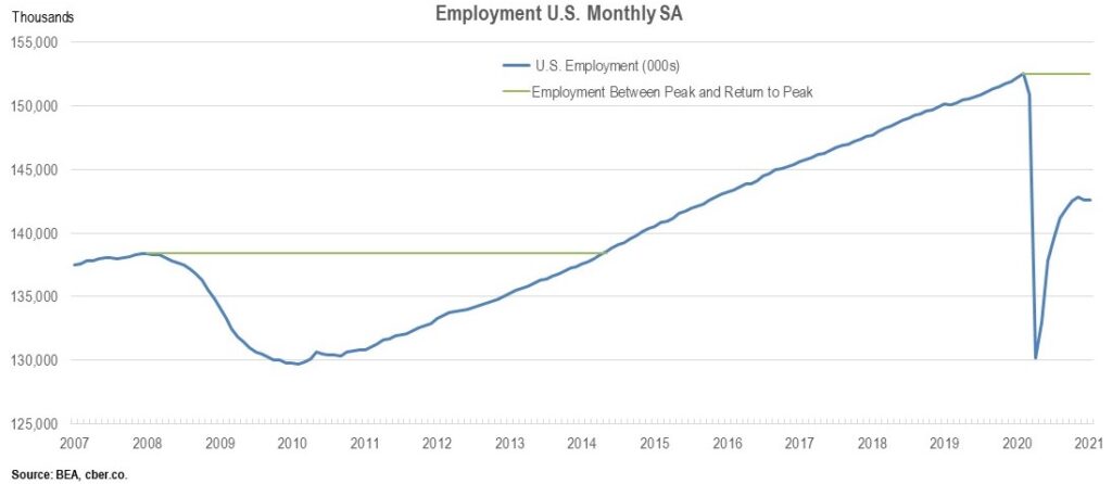
U.S. employment peaked in January 2008. As the financial crisis snowballed, U.S. employment declined for 25 months. This declined was longer than the COVID-19 recession, but not as deep.

At the trough in 2010, U.S. employment was 93.7% of the January 2008 total. It took 51 months of job recovery to return to the January 2008 level. The combined length of the employment decline and recovery was 76 months.

The recovery from the COVID-19 recession will be in Q4 of 2022 or Q1 of 2023. The estimated time of recovery from the trough will be 2.5 to 3.0 years. The total estimated time of recovery from the previous peak is approximately 31 to 37 months.

There are many potential headwinds. Keep your fingers crossed.

Panthers vs. Broncos – The Economics of the Two Cities

On February 7, Super Bowl 50 will feature the Panthers vs. Broncos. Without a doubt, most Coloradans think the outcome of the game is a foregone conclusion. Some fans have painted their houses and dyed their hair orange and blue because they know the Broncos will win.

One of the fun parts about the hype of Super Bowls is the statistics associated with the big game. For example, CBS Sports has reported that on Super Bowl Sunday fans will drink 325.5 million gallons of beer and eat 1.25 billion chicken wings. Really?

From an economic perspective how do the city of Charlotte and Denver match up?

The following table includes economic data from the Bureau of Census Quickfacts (2/14/2016) comparing the city of Denver and Charlotte.

Statistic Denver Charlotte Winner
Population estimates, July 1, 2014 663,862 809,958 Charlotte
Population, % change – 4/1/10 to 7/1/14 10.6% 10.1% Denver
Owner-occupied housing unit rate, 2010-2014 49.7% 55.4% Charlotte
Median value of owner-occupied housing, 2010-2014 $257,500 $170,200 Charlotte
Median selected monthly owner costs -with a mortgage, 2010-2014 $1,592 $1,416 Charlotte
Median gross rent, 2010-2014 $913 $902 Charlotte
Households, 2010-2014 271,054 298,815 Charlotte
High school graduate or higher, percent of persons age 25 years+, 2010-2014 85.6% 88.1% Charlotte
Bachelor's degree or higher, percent of persons age 25 years+, 2010-2014 43.7% 40.7% Denver
Persons without health insurance, under age 65 years, percent 17.6% 18.9% Denver
Mean travel time to work (minutes), workers age 16 years+, 2010-2014 24.5% 24.5% Tie
Median household income (in 2014 dollars), 2010-2014 51,800 53,274 Charlotte
Per capita income in past 12 months (in 2014 dollars), 2010-2014 34,423 31,844 Denver
Persons in poverty, percent 18.3% 17.3% Charlotte

Charlotte is the larger of the two cities, but recently Denver has grown at a slightly faster pace. Housing and rent are less expensive in Charlotte and the city has a higher owner-occupied housing rate. Charlotte has a higher percentage of high school degrees, but Denver wins the battle for bachelor’s degrees. Charlotte has a higher median household income, but Denver has a higher per capita income. Charlotte has a higher percentage of people without health insurance, but Denver has a higher rate of persons in poverty.

Both are prosperous cities. Panthers vs. Bronocs. Game on!

cber.co 2016 Colorado Economic Forecast – Solid Growth

Last week, cber.co released its Colorado economic forecast for 2016. As is the case with most forecasts, the primary focus of the Colorado forecast is employment. As economic developers say, “it all starts with a job.”

Each year the forecast provides an optimistic, pessimistic, and most likely scenario.

The 2016 optimistic scenario calls for:
• U.S. Real GDP growth will be greater than 2.6%.
• Colorado will add more than 73,000 workers, the rate of job growth will be greater than 2.9%.

The projected likelihood of this scenario is 18%. The Colorado economy has experienced solid job growth since 2012; however, given the slowdown in the global economy and the lower price of oil, it is unlikely the state will experience accelerated growth.

The pessimistic scenario calls for:
• U.S. Real GDP growth will be less than 2.3%.
• Less that 67,000 Colorado workers. Job growth will be less than 2.7%.
The projected likelihood of this scenario is 22%. While the global and U.S. economies are expected to see slight growth in output, the Colorado economy could be derailed if the price of oil stays low and the global economy slows further.

The most likely scenario calls for:
• U.S. Real GDP will be 2.3% to 2.7%.
• The U.S. will add at least 2.7 million workers.
• Colorado will add 1.8% of total U.S. jobs added.
• Colorado will add 67,000 to 73,000 workers, job growth will be 2.7% to 2.9%.

Despite downside risks there is a 55% likelihood this forecast will occur. Since 2012 growth has been steady and broad-based. Much of the growth has been in sectors such as tourism, which have an indirect link to the extractive industries.

The bottom line – look for continued job growth in Colorado, but at a slower rate than 2015.

For additional information about the 2016 cber.co Colorado Economic Forecast click here.

colorado economic forecast

Which has the Top Economy – Colorado, Utah, Washington?

There are frequent references in the local media about how Colorado is one of the top state economies in the country. And it is!

There are many metrics that can be used to compare state economies. The two best metrics are the growth rates for Real GDP and employment. In this post we look at these metrics from 2005 to the present for Colorado, Utah, Washington and the U.S.

Employment
• Washington has the greatest number of employees, followed by Colorado.
• Utah had the highest rate of employment growth of the three states. Colorado and Washington have grown at similar rates; however, Washington’s rate of growth has been off a larger base of employment.
• Employment for all three states has grown at a faster rate than the U.S. That rate of growth has accelerated since 2010 for all three states.

Colorado Utah Washington

Real GDP
• Washington has the largest GDP, followed by Colorado.
• The Real GDP for all three states has grown at a higher rate than the U.S.
• Utah had the fastest rate of Real GDP growth from 2005 to present followed by Washington. Colorado is third.
• Since the end of the recession the GDP for all three states has grown at a faster rate than the United States. Colorado had the fastest rate of Real GDP growth from 2013 to present because of the rapid growth in the extractive industries. That rate of growth is likely to decrease in 2015 and beyond as a result of challenges facing the oil and gas industry caused by lower oil prices.

Colorado Utah Washington

Based on these metrics Washington has the largest economy and Utah is growing at a faster rate than the other two states. The strengths of the economies in Utah, Washington, and Colorado make them great places to live, work, and play. Here’s to a prosperous year for all three states in 2016.

If the Economy is Doing so Well, Why Doesn’t it Feel More Robust? -Take II

In the previous blog post, the topic of the economic recovery was discussed. Although it has been a solid recovery, why doesn’t it feel more robust?

The 2007 recovery was atypical in that it occurred over a period of years, as opposed to months. As a result Colorado posted accelerating job growth for four consecutive years. Essentially, the recovery from the recession was weak and gradual. At no point has the state reached a point where public and private leaders could really say, “We have arrived.”

At the national level, the U.S. will add 3.0 million jobs in 2015. Yet, the focus is on the slowdown of the global economy, not the fact that 2015 will be the fifth consecutive year of solid job growth.

Nationally, GDP growth has been subpar. It is hard to get excited when the rate of Real GDP growth is 2.0% to 2.5%. Consumer spending has increased at a similar anemic rate. In other words consumers have remained cautious, as if they are always looking over their shoulder.

The construction industry is “booming” and there is a shortage of trained workers. At the same time, the growth of the industry pales when compared to the 2000s. The good news is that housing has been built on an “as needed basis” and the chance of being overbuilt is slim.

During the recovery period, the state has suffered natural tragedies. There were multiple severe forest fires in several parts of the state, as well as flooding and drought. That was taxing on the state – fiscally and psychologically. Fortunately, Coloradans have remained resilient.

Lower oil prices have dampened growth in parts of the state that had previously experienced strong growth. It is easy to forget the risk associated with the extractive industries until the price of the commodities (oil, molybdenum, coal) drops precipitously or regulations are established that eliminate demand for these commodities.

Then there is the state government… The legislature has focused on social issues for the past couple of sessions – and that is not bad. Some feel insufficient time and resources were spent addressing issues that could improve the state’s ability to conduct business.

At one point, there was sufficient discourse to cause several counties to threaten secession from the state. At times, state government seemed dysfunctional over the past five years.

State government faces a new problem – the state economy is on solid footing and the state will generate record levels of revenue, yet the legislature will be forced to make cuts to key service areas. This conundrum is caused by the combination of Amendment 23, the Gallagher Amendment, TABOR, the initiative process, and Medicare obligations. It is difficult for legislators to govern the state in a way they feel is appropriate.

Despite the challenges and angst created by the items mentioned above, the growth of Colorado’s economy has exceeded the growth of the U.S. economy in many key areas (rate of job growth, rate of population growth, growth of Gross Domestic Product).

Unfortunately, the picture hasn’t always been rosy for the past five years, despite the many great things that have happened.

If the Economy is Doing so Well, Why Doesn’t it Feel More Robust?

The Great Recession has been over for five years, but in many ways the economy still feels like we are still in the recovery stages.

In 2001 the business cycle was coming to an end when 9/11 exacerbated the situation. Workers in most sectors were touched by the recession. Fortunately, we could blame the downturn on the terrorists.

The country rallied, and with fiscal policies such as zero percent financing we recovered – some would say it was a false recovery because we stole sales from the future. By 2007 we were confident that all would be well, but that didn’t turn out to be the case.

In both recessions many families were hit hard, regardless of race, job title, or income level. In some cases one or both spouses lost their job, establishments went out of business, people had their houses foreclosed on, and there was no place to hide. Both recessions touched nearly everyone and the fact they were back-to-back doubled the pain.

In 2007 most economists did not see the 2007 recession coming and when they realized something was wrong, they failed to acknowledge that it was for real. In fact some of the state’s leading economists were in denial. (It is almost funny to re-read newspaper articles and emails from that era talking about the economy.)

In retrospect there were some small signs pointing to the 2007 recession, such as declines in financial employment. These signs weren’t sufficient to make anyone believe a major downturn was impending. For the most part, the public did not have access to the data and information that caused the problem. Many of those who had access to the information may not have understood the ramifications of what was actually happening. In some cases those who had access to the information conveniently ignored it. As business leaders and the public learned about the cause of the recession some felt betrayed by what happened. They had a right to be upset because the 2007 recession was not part of a normal business cycle. It was self-inflicted.

Psychologically the “back-to-back” recessions changed the structure of the way companies do business. Companies had to find ways to be successful with fewer employees. As a result they became more efficient and hired fewer workers during the recovery.

It was difficult for some of the laid off workers to come to terms with the realization they wouldn’t have a job waiting for them when things got better. It was tough for older workers to be ungraciously kicked off the payrolls. At the same time, several graduating classes of college students, with hefty student loans, were passed over because there were no jobs for them.

Many of the workers who held onto their jobs felt both blessed and cursed. They were fortunate to have a job, yet at times they were taken advantage of (minimal or no pay increases, reduced benefits, longer hours, more responsibilities). Work became a necessary burden for many.

As a result of the “back-to-back” recessions consumers changed spending patterns, particularly in retail. Many people have been more discrete with their spending, they may not spent as much they once spent, and they tend to wait for items to be on sale before they purchase them. Adults with family members who had experienced the Great Depression may have benefitted from their experiences. As the Rolling Stones said, “You can’t always get what you want, but if you try sometime you find you get what you need.”

Economists are partially to blame for the feeling the economy does not feel more robust. They continually refer back to the recession in their charts and their discussions. By continuing to refer to the recession, economists are continually reminding people how bad the economy was just a few years ago. It is difficult to feel the economy is robust when you are always looking over your shoulder.

Stock Market Cycles and Elections

James Carville coined the phrase, “It’s the Economy, stupid” to remind voters in the 1992 presidential campaign about the importance of the economy when casting their ballot.

For many years prior to 1992, members of the executive and legislative branches realized they had a better chance of getting re-elected if they influenced fiscal policy (taxes, incentives, wage and job increases, etc.) to create the perception their leadership was responsible for a healthy economy.

As a result of their manipulation, four-year stock market cycles evolved. The cycle assumes companies, and thus investments, have a stronger performance in the second half of a president’s term and a weaker performance in the first half.

This short analysis looks at the performance of the Standard & Poor’s 500 Index (S&P 500) for the presidential terms from 1952 to 2016. Obviously the period 2013 to 2016 is still in progress; however, a case can be made that the current bull market will not follow the above mentioned trends.

Fifteen stock market cycles were evaluated. The average time from peak to peak was 1,534 days or 4.2 years and the average time from trough to trough was 1,509 days or 4.1 years.

The two tables that follow look at the peaks and troughs and the year they occurred for each of the presidential terms.

The first table looks at the peaks.
• Year 1 – 3 peaks.
• Year 2 – 3 peaks.
• Year 3 – 2 peaks.
• Year 4 – 7 peaks.
Sixty percent of the peaks occurred during the second half of the presidential term.

Presidential Term Date S&P Change Up Annualized % Change Up # of Days Up Year Up
1953-1956 9/14/1953 22.71
8/3/1956 49.64 26.93 31.10% 1,054 Year 4
1957-1960 10/22/1957 38.98
1961-1964 12/12/1961 72.64 33.66 16.20% 1,512 Year 1
6/26/1962 52.32
1965-1968 2/9/1966 94.06 41.74 17.60% 1,324 Year 1
10/7/1966 73.2
11/29/1968 108.37 35.17 20.00% 784 Year 4
1969-1972 5/26/1970 69.29
1973-1976 1/11/1973 120.24 50.95 23.30% 961 Year 2
10/3/1974 62.28
9/21/1976 107.83 45.55 32.10% 719 Year 4
1977-1980 3/6/1978 86.9
11/28/1980 140.52 53.62 19.20% 998 Year 4
1981-1984 8/12/1982 102.42
1985-1988 8/25/1987 336.77 234.35 26.60% 1,839 Year 3
12/4/1987 223.92
1989-1992 7/16/1990 368.95 145.03 21.00% 955 Year 1
10/11/1990 295.46
1993-1996 2/2/1994 482 186.54 15.90% 1,210 Year 2
4/4/1994 438.92
1997-2000 7/17/1998 1,186.75 747.83 26.10% 1,565 Year 4
8/31/1998 957.28
3/24/2000 1,527.45 570.17 34.80% 571 Year 4
2001-2004 10/9/2002 776.76
2005-2008 5/19/2008 1,426.63 649.87 11.40% 2,049 Year 4
2009-2012 3/9/2009 676.53
11/3/2010 1,363.61 687.08 52.70% 604 Year 2
8/2/2011 1,099.23
2013-2016 5/21/2015 2,130.82 1,031.59 19.00% 1,388 Year 3

The second table looks at the troughs..
• Year 1 – 3 troughs.
• Year 2 – 10 troughs.
• Year 3 – 2 troughs.
• Year 4 – 0 troughs.
About 87% of the troughs occurred during the first half of the presidential term. This suggests that fiscal policy in the third or fourth year of a presidential term may have prevented or postponed economic weakness for that year, but it mostly likely have kicked the can forward to the first half of the subsequent presidential term. In some cases pushing the weakness forward had a detrimental impact on the economy.

Presidential Term Date S&P Change Down Annualized % Change Up # of Days Down Year Down
1953-1956 9/14/1953 22.71 Year 1
8/3/1956 49.64
1957-1960 10/22/1957 38.98 -10.66 -18.00% 445 Year 1
1961-1964 12/12/1961 72.64
6/26/1962 52.32 -20.32 -45.70% 196 Year 2
1965-1968 2/9/1966 94.06
10/7/1966 73.2 -20.86 -31.70% 240 Year 2
11/29/1968 108.37
1969-1972 5/26/1970 69.29 -39.08 -26.00% 543 Year 2
1973-1976 1/11/1973 120.24
10/3/1974 62.28 -57.96 -31.70% 630 Year 2
9/21/1976 107.83
1977-1980 3/6/1978 86.9 -20.93 -13.80% 531 Year 2
11/28/1980 140.52
1981-1984 8/12/1982 102.42 -38.1 -16.90% 622 Year 2
1985-1988 8/25/1987 336.77
12/4/1987 223.92 -112.85 -77.10% 101 Year 3
1989-1992 7/16/1990 368.95
10/11/1990 295.46 -73.49 -60.60% 87 Year 2
1993-1996 2/2/1994 482
4/4/1994 438.92 -43.08 -42.90% 61 Year 2
1997-2000 7/17/1998 1,186.75
8/31/1998 957.28 -229.47 -82.50% 45 Year 2
3/24/2000 1,527.45
2001-2004 10/9/2002 776.76 -750.69 -23.30% 929 Year 2
2005-2008 5/19/2008 1,426.63
2009-2012 3/9/2009 676.53 -750.1 -60.40% 294 Year 1
11/3/2010 1,363.61
8/2/2011 1,099.23 -264.38 -25.10% 272 Year 3
2013-2016 5/21/2015 2,130.82

The following three charts show the daily performance of the S&P 500 for 1953 to 1976, 1973 to 1996, and 1993 to 2016.

The average number of days for periods of growth were longer than the downturns, 1,169 days compared to 357 days. The moral of the story is that growth occurs steadily over time, but losses are usually quick and painful.

stock market cycles and elections

In addition, the average increase in the S&P 500 was 300 points during positive cycles, compared to 173 points for the down cycles.

stock market cycles and elections

The most severe absolute decline in the S&P 500 ended on March 9, 2009 when the index closed at 676.53. Over the previous 294 days the index plummeted 750.10 points, an annualized change of -60.4%.

The current bull market will most likely be the strongest for the period 1952-2016. The bull market that started on March 9, 2009 was also notable. It ended on November 3, 2010 when the S&P 500 closed at 1,363.61. Over 604 days the index recaptured 687.08 points that it had lost, an annualized gain of 52.7%.

stock market cycles and elections

Expect Solid Growth in Colorado Wage and Salary Employment

The U.S. economy remains on solid footing  in anticipation of the upcoming release of BLS Colorado wage and salary employment data.

U.S. Employment and GDP

Earlier this month BLS reported the U.S. added 126,000 jobs in March compared to February. This was the weakest level of month-over-previous-month job growth for the seasonally adjusted data since 2013. Despite the slower rate of growth for March 2015, U.S. employment for March is about 2.29 million jobs greater than March 2014..

Currently, Colorado wage and salary employment is about 1.8% of the U.S. total. About 2.8% of U.S. job growth can be attributed to Colorado.

Most economists think U.S. Real GDP growth will be in the neighborhood of 2.5% to 3.0% this year. This past week The Conference Board bumped its 2015 projection for the U.S. output growth up to 2.9% based on projections for stronger personal consumption. This is notable given their conservative estimates over the past ten years. Meanwhile, other economists have bumped their forecasts down to the range of 2.5% to 3.0%

Stronger output growth should translate into a greater number of wage and salary workers. In other words, the slower rate of U.S. job growth in March appears to be a glitch rather than the start of a downward trend. The strong rate of U.S. job and output growth will ensure that in the short term Colorado with continue to add jobs at a rate similar to the past twelve months.

U.S. and Colorado Unemployment Rates

In March the U.S. unemployment rate remained steady at 5.5%, but down from 6.6% a year ago.

The U.S. Congressional Budget Office has indicated the natural rate of unemployment is currently 5.2%. The natural rate is the point of equilibrium or the rate at which an economy will operate most efficiently.

When the unemployment rate drops below the natural rate there will be upward wage pressures and companies will be challenged to find qualified workers. The economy will operate inefficiently for different reasons than when the rate of unemployment is above the natural rate.

In Colorado, the February unemployment rate of 4.2% was well below the U.S. rate. Some Colorado industries are currently experiencing symptoms of an economy that is operating below the natural rate of unemployment. They are experiencing difficulty finding qualified workers in select occupations. In addition, there are upward wage pressures in industries such as construction and agriculture. Anecdotal evidence suggests some companies are not able to find workers even when they pay higher wages.

The state’s rate of unemployment is expected to remain below 4.5% in the near-term, although there are concerns the layoffs caused by lower oil prices will cause an increase in the unemployment rate. At the state level the direct impact of oil and gas layoffs may not have a major impact on total state employment and unemployment data, but it will definitely affect regions where the oil and gas industry has played a significant role in the economy, such as Weld and Garfield counties.

Expect continued solid growth in Colorado wage and salary employment in the short-term.

2015 cber.co Forecast – Fine Tuning the Volatile Category

In preparing its annual forecast, cber.co divides the NAICS sectors into three categories. This portfolio approach makes it easy to see that some sectors consistently create jobs at a higher rate of growth, some show solid growth, and others are more volatile. Ultimately, the volatile category tends to have a greater influence on the magnitude of change in total job growth than the sectors with steady growth. In March 2015 BLS released its benchmark revision of the 2014 data. The changes were more significant than usual.

As a result  the 2015 cber.co forecast was fine-tuned to have a better understanding of categories and sectors that were driving the economy. This brief discussion highlights the revisions to the 2015 cber.co forecast. This post will evaluate the Volatile Category.

The Volatile Category

Over the past two decades the sectors listed below were the primary source of volatility in total employment.

The sectors are:

  • Natural Resources and Mining
  • Construction
  • Manufacturing
  • Transportation, Warehousing, and Utilities
  • Employment Services
  • Financial Activities
  • Information
  • Federal Government

Total employment for this category was:

  • 1994  625,400 workers, 35.6% of total employment
  • 2004  716,000 workers, 32.8% of total employment
  • 2014  713,000 workers, 29.0% of total employment

2015 cber.co forecast

Estimated Job Growth

As can be seen below there is a significant difference between the original estimates for 2014 (January 11) and Benchmark revisions for 2014 (March 27). BLS significantly underestimated growth in this category in 2014.

The original Volatile Category estimates/forecast (January 11 Forecast) was + 23,000 to 27,000 Employees.

  • 19,800 jobs added in 2013
  • 25,600 jobs added in 2014
  • 706,100 employees in 2014

In 2015 between 23,000 and 27,000 jobs will be added, at a rate of 3.3% to 3.7%. This rate of growth is slightly slower than 2014.

The updated Volatile Category estimates/ forecasts, after benchmark revisions (March 27 Forecast) was + 23,000 to 27,000 Employees.

  • 22,200 jobs added in 2013
  • 30,000 jobs added in 2014
  • 713,000 employees in 2014

In 2015, between 23,000 and 27,000 workers will be added at a rate of 3.2% to 3.8%. Despite the significant underestimate in 2014, the forecast for 2015 was unchanged.

The recalibration of the 2015 forecast resulted in the following changes:
• The Strong Growth Category was revised upward by 4,500.
• The Solid Growth Category was revised downward by 1,500.
• The Volatile Category remained unchanged.
• The net change to the 2015 forecast was an upward revision of 3,000; however, the 2015 forecast is for total growth slightly below the 2014 total.

The change in the mix of jobs being added is equally as important as the change in the number of jobs being added. For further information on the cber.co forecasts click here.

2015 cber.co forecast


2014 Unemployment Rate – Challenges and Positives for 2015

On March 4, the Bureau of Labor Statistics released its annual unemployment data for Colorado. The 2014 unemployment rate for Colorado was 5.0%, down from 6.8% in 2013. The average number of unemployed decreased from 189,023 in 2013 to 141,387 in 2014.

With that as a background, some of the challenges and positives facing the economy are listed below.

Employment in Colorado has increased at a modest and manageable rate for the last two years. A similar level of growth is expected in 2015, but there will be some challenges.
• The decline in the price of oil has begun to hit Colorado producers. The breakeven point for the Niobrara is in the $65 to $70 range. Several companies have announced significant layoffs.
• In addition to the drop in the price of oil, demand for Colorado coal declined in 2014. Coal is a major driver of several rural economies throughout the state. With the decline in demand, many communities are fine tuning their economic development strategies to diversify their economies.
• Colorado’s rate of inflation is more than a point higher than the rate for the U.S. (The Denver-Boulder-Greeley index is used as a proxy for the state). Last year it was 1.6% for the U.S., while it was 2.8% for Colorado. The rapidly appreciating prices of housing in Denver and many parts of the state are largely responsible for the gap in inflation between the state and the nation.
• Rising home prices are a two-edged sword. They benefit the home owners but may be detrimental to prospective buyers. In parts of the Front Range, there is solid demand and low inventories for certain types of housing, particularly at the lower end. Affordable and attainable housing are in high demand.

On the other hand the state has many positives:
• Nationally, jobs are being added at rate that is accelerating slightly. That bodes well for Colorado.
• The decline in oil and gas prices has increased disposable income slightly, about $50 for 2014 and $500 to $700 for 2015.
• Rising home prices will be beneficial to Colorado. Homeowners are more confident if they feel the value of their home is increasing. As a result they may spend more. Rising property values directly benefit the coffers of local governments and school districts.
• After a slowdown in 2014, Wall Street is enjoying a bull market. This in turn creates wealth and increases greater consumer and business confidence.
• Unemployment is expected to remain below 5.0% throughout 2015. As a result wage pressures will become a bigger issue in more occupations and industries. This is great for workers, particularly if their increases exceed Colorado’s rate of inflation (2.8% in 2014). Wage increases that exceed the rate of inflation will serve as a form of stimulus to the economy because workers will have greater confidence and more to spend. In turn, education and state and local government will be able to more fully fund programs that have been underfunded in the past.
• Because the decline in the price of oil is a global issue, oil and gas employees may not be able to move to other states or countries to find work. With the Colorado unemployment in the range of 4.0% some of these workers may be able to stay in-state and work in construction, manufacturing or other positions.
• Colorado has experienced another first-rate ski season, with an added benefit of hosting the 2015 FIS Alpine World Ski Championships in Vail. The event showcased the state to 700 athletes from more than 70 nations.
• The spring snow storms significantly increased snowpack levels in many parts of the state; however, additional snow is needed. Water in critical for all aspects of Colorado’s economy. While the snow is often viewed as an inconvenience to those along the Front Range, it is essential to have good snow pack in our mountains and counties where agriculture dominates the local economy.
• The sectors that have driven the economy over the past two years are construction; healthcare; accommodations and food services; retail trade; and professional, scientific, and technical services (PST). These sectors are expected to account for about 60% of the job growth in the state in 2015. There will admittedly be challenges in the extractive industries; however, they will have a minor impact on the growth of the state’s top five sectors for job growth.

As Colorado addresses these challenges and positives, job growth in 2015 is expected to be at or slightly less than the rate for 2014.